How Do You Know Where the Break Is?
An optical power meter tells you how much loss there is. It cannot tell you where. Knowing that a 3 km span lost more than it should does not tell you where to dig.
An OTDR answers that question.
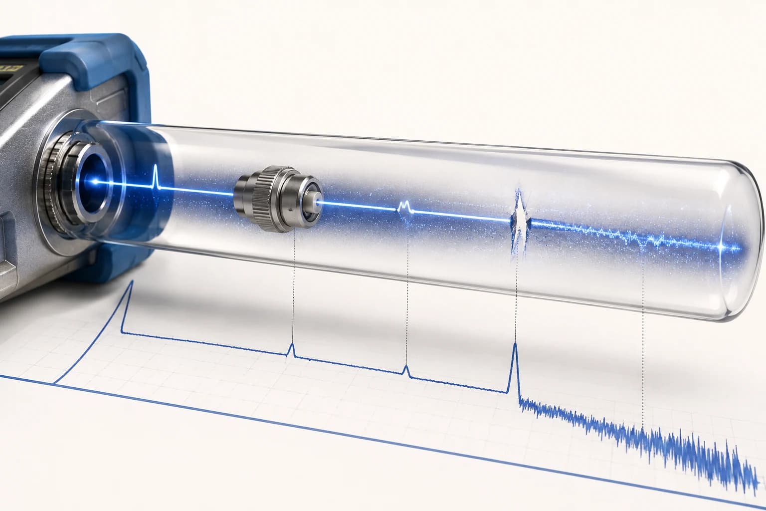
The Principle — Send Light, Watch What Comes Back
An OTDR (Optical Time Domain Reflectometer) launches short optical pulses into the fiber and records the returning light against time.
As light travels down the fiber, a small fraction scatters in all directions, and some of that scatter returns along the original path. At points where the refractive index changes abruptly, such as a connector or a break, the reflection is much stronger.
Knowing the return time gives you distance. The result is a graph with distance on the horizontal axis and signal level on the vertical axis. That is the OTDR trace.
What the Trace Tells You
A healthy trace is a gentle downward slope from left to right, caused by the attenuation of the fiber itself. The features sitting on that slope are the information.
A Step Down with No Spike — Fusion Splice
The signal drops without any reflection. A fusion splice fuses the two fibers into one, so the index change is small and there is almost nothing to reflect.
The height of the drop is the loss of that splice. Under 0.1 dB is good. Above 0.3 dB, it is usually worth redoing.
A Spike Then a Drop — Connector
A sharp peak appears, because the connector interface reflects strongly. The amount the signal settles lower after the peak is the loss.
The size of the reflection is itself a signal. An unusually large reflection often means the connector is contaminated or not fully mated.
A Vertical Drop to the Noise Floor — End or Break
The trace falls to the bottom and only noise follows. The fiber ends there.
The question is whether that is the designed end or a break. Distance settles it. If the drawing puts the termination at 3.2 km and the trace ends at 1.7 km, then 1.7 km is your fault location.
A Spike with No Loss
A mechanical splice or connector that reflects strongly but costs little loss. It is not a problem today, but strongly reflective points tend to degrade over time, so it is worth recording.
Settings Change the Answer
This is where newcomers most often go wrong. The same fiber measured with different settings produces different results.
Pulse Width
Short pulses resolve nearby events precisely. Long pulses reach further but smear detail.
Short — good resolution, able to separate two closely spaced events. Limited range. Long — reaches the far end. Closely spaced events merge into one.
Which is why, in practice, you do not measure only once. Use a short pulse for the near section and a longer one for the whole span, two or three captures in total.
Distance Range
Set it shorter than the actual span and the far end is cut off. Set it far too long and resolution suffers. Roughly 1.5 to 2 times the expected length works well.
Averaging Time
Longer averaging suppresses noise and produces a cleaner trace. Rush it and small splice losses disappear into the noise.
Dead Zone — The Part You Cannot See
Connect an OTDR directly to the fiber and the first few tens of meters are invisible. The strong reflection from the first connector briefly saturates the receiver. That region is the dead zone.
This is why the field practice is to insert a launch cable, a dummy fiber of a few hundred meters, ahead of the span. The dead zone then falls inside the launch cable, and the first real connector can be measured properly.
Measuring without a launch cable and concluding that "the first event is not visible" gets it backwards. The event is there; the instrument simply cannot see it yet.
Why Bidirectional Measurement Matters
Measure from one end only and splice loss can read lower than reality, and sometimes even negative, as if the splice produced gain. Light does not gain energy at a splice.
The cause is that the two fibers being joined have slightly different backscatter characteristics. Splice two dissimilar fibers and one direction underestimates the loss while the other overestimates it.
Measuring from both ends and averaging gives the true value. That is precisely why acceptance testing calls for bidirectional measurement.
Field Sequence
A typical order of work after a fault report:
- Measure optical power — is the link dead, or merely weak?
- Clean connectors and remeasure — the most common cause, and the fastest to clear.
- Run the OTDR — localize by distance and event signature.
- Compare against the drawing — convert measured distance to a physical location. Because of slack coils and duct routing, fiber length and ground distance are not the same.
- Verify on site and repair.
Skip step 4, trust the raw distance, and you will excavate in the wrong place. Slack stored at each enclosure adds up to a meaningful error over a long span.
Summary
- An OTDR maps loss against distance using backscattered light.
- Splices drop without reflecting, connectors spike then drop, breaks fall to the noise floor.
- Pulse width, range and averaging change the result. Never rely on a single capture.
- Without a launch cable the near end is invisible, and splice loss is only accurate when measured both ways.
- Measured fiber distance is not ground distance. Comparing against the drawing is the last step before you dig.